简介
Allen Brain Atlas项目是一个公开可用的人脑基因表达信息的在线资源,已有数百篇文章采用了该数据库。基因组学的数据主要是采用了microarray(基因芯片)检测基因序列表达的同时保留空间信息的一种方式。
具体的细节可以参考官网的documentation
部分需要了解的名词:
- 转录组学:简单理解,研究RNA表达的,由于DNA需要表达成蛋白质才能够起作用,而RNA是翻译成蛋白质所必须的,故而对RNA进行研究
- 空间转录组学:在研究RNA表达的同时保留空间信息,即知道在大脑的哪个地方表达了哪个基因
- RNA-seq:RNA sequencing,即RNA测序
- 基因表达谱:某一状态下的细胞或组织的基因表达信息
- 基因表达阵列:包含样本和基因表达值的矩阵
- 基因表达:由DNA的编码部分转录成RNA或转录并翻译成蛋白质的过程及结果
- 转录:DNA->RNA,范围上绝大部分RNA∈DNA
- 翻译:RNA->蛋白质,范围上蛋白质∈RNA
- 探针:只结合某一段基因的序列,可以特异性识别某个基因
数据
基本信息
基因组数据
共包含来自6个患者的3702个不同空间的样本的基因芯片结果,每个基因表达谱包含超过62,000个基因探针的信息,93%的已知基因至少有两个探针。
已下载至:/data/disk1/zhangyi/Allen
官网提供三种基因组数据的下载
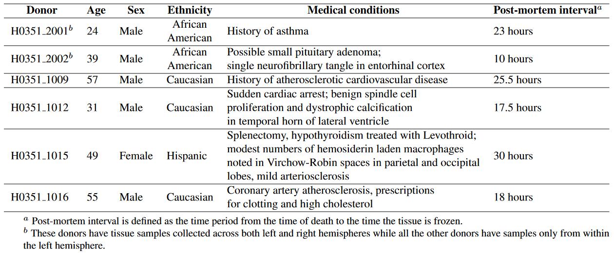
- 经过标准化的基因芯片数据集(in March 2013),包含全部的六个患者的基因表达阵列,ID:H0351.2001, H0351.2002, H0351.1009, H0351.1012, H0351.1015, H0351.1016.
- RNA-seq数据集,通过测序技术得到的两个患者的基因表达量,ID:H0351.2001, H0351.2002.
- 旧的基因芯片数据集,ID:H0351.2001, H0351.2002, H0351.1009, H0351.1012.
具体的标准化过程可以参考技术白皮书, Microarray Data Normalization.
下图是以CLRN1基因在不同样本中的分布示意图
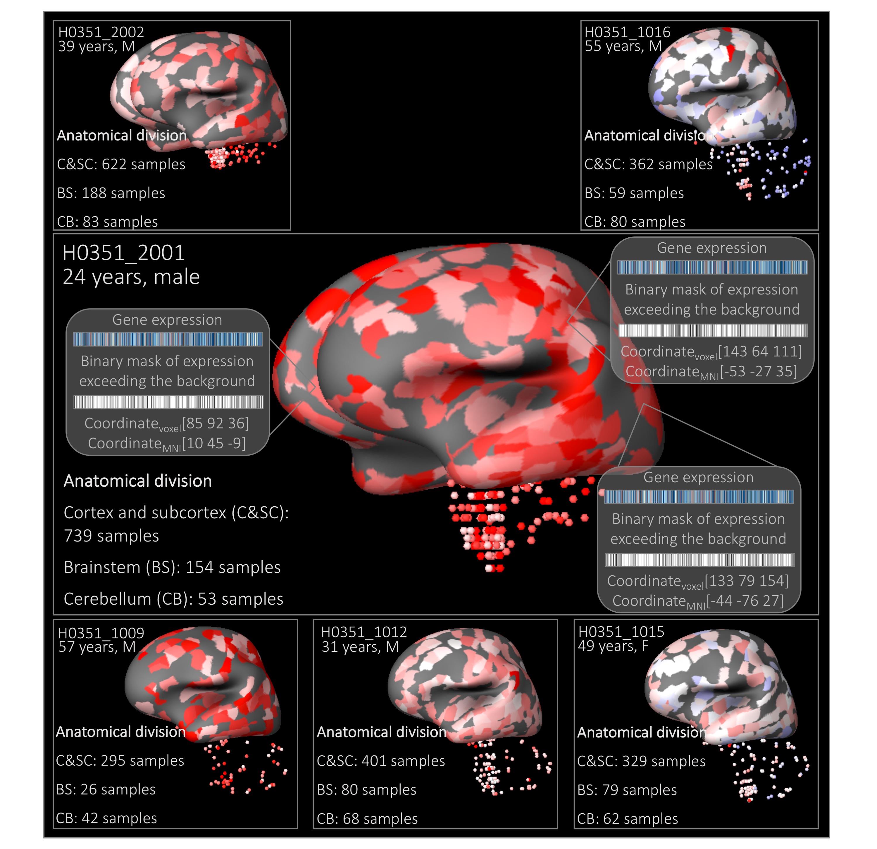
颜色代表基因表达的水平,红色为高,cortex and subcortex (C&SC), brainstem (BS) and cerebellum (CB)
影像学数据
-
H0351.1009 / H0351.1012
- T1-weighted MPRAGE structural MRI with 0.98 x 0.98 x1 mm voxels, three-dimensional acquisition, three averages, TI = 900 ms, TR = 1900 ms, TE = 3.03 ms, 9° flip angle, image matrix = 256 x 256 x 176.
- T2-weighted images were taken in three-dimensions with 0.98 x 0.98 x 1 voxels, TR = 3200 ms, TE = 449 ms, 120° flip angle, image matrix = 256 x 256 x 192 voxels
- FLAIR images acquired in 0.98 x 0.98 mm axial slices and 5 mm slices, TI = 2500 ms, TR= 10000 ms, TE= 73 ms, 150° flip angle, image matrix = 256 x 256 x 20 voxels.
- T2-weighted gradient echo images taken in axial slices with 0.72 x 0.72 mm and 5 mm slices, TR = 889 ms, TE = 18 ms, 60° flip angle, image matrix = 320 x 290 x 24 voxels.
-
H0351.1015 / H0351.1016
- T1-weighted MPRAGE structural MRI with 0.98 x 0.98 x1 mm voxels, three-dimensional acquisition, three averages, TI = 900 ms, TR = 1900 ms, TE = 2.63 ms, 9° flip angle, image matrix = 256 x 256 x 176.
- T2-weighted / FLAIR / T2-weighted gradient echo同上
-
H0351.2001
- T1-weighted MPRAGE structural MRI with 1 mm isotropic voxels, three-dimensional acquisition, three averages, TI = 900 ms, TR = 1900 ms, TE = 2.63 ms, 9o flip angle, image matrix = 256 x 192 x 256.
- T2-weighted images were taken in three-dimensions with 0.9 mm isotropic voxels, TR = 3210 ms, TE = 540 ms, 120o flip angle, image matrix = 224 x 256 x 160 voxels.
- DT images taken in 64 directions using an Echo Planar Imaging sequence taken in 2 mm axial slices with 1.875 x 1.875 mm in plane voxels, TR = 9300 ms, TE = 94 ms, 90o flip angle, image matrix = 128 x 128 x 68.
- FLAIR images acquired in 0.86 mm x 0.86 mm axial slices and 5 mm slices with a 1 mm gap, TI = 2500 ms, TR= 8000 ms, TE= 67 ms, 170o flip angle, image matrix = 208 x 256 x 26 voxels.
- T2-weighted gradient echo images taken in axial slices with 0.86 mm x 0.86 mm and 5 mm slices, TR = 613 ms, TE = 20 ms, 20o flip angle, image matrix = 256 x 256 x 26 voxels
- Inversion recovery images taken with sagittal sections with 0.86 mm x 0.86 sagittal sections and 4 mm slices, TI = 185 ms, TR = 5523.2 ms, TE = 62 ms, 170o flip angle, image matrix = 248 x 256 x 33 voxels.
-
H0351.2002
- T1-weighted MPRAGE structural MRI with 1 mm isotropic voxels, three-dimensional acquisition, three averages, TI = 900 ms, TR = 1900 ms, TE = 2.63 ms, 9o flip angle, image matrix = 256 x 192 x 256.
- T2-weighted images were taken in three-dimensions with 0.9 mm isotropic voxels, TR = 3200 ms, TE = 535 ms, 120o flip angle, image matrix = 224 x 256 x 160 voxels.
- DT images taken in 64 directions using an Echo Planar Imaging sequence taken in 5mm axial slices with 1.875 x 1.875 mm in plane voxels, TR = 9300 ms, TE = 94 ms, 90o flip angle, image matrix = 128 x 128 x 24.
- FLAIR images acquired in 0.94 mm x 0.94 mm axial slices and 5 mm slices with a 1 mm gap, TI = 2000 ms, TR= 8000 ms, TE= 67 ms, 170o flip angle, image matrix = 208 x 256 x 24 voxels.
- T2-weighted gradient echo images taken in axial slices with 0.94 mm x 0.94 mm and 5 mm slices, TR = 665 ms, TE = 20 ms, 20o flip angle, image matrix = 256 x 256 x 24 voxels.
- Inversion recovery images taken with sagittal sections with 0.86 mm x 0.86 mm sagittal sections and 3 mm slices, TI = 185 ms, TR = 4230 ms, TE = 62 ms, 170o flip angle, image matrix = 248 x 256 x 25 voxels.
在线工具
1. MicroArray(基因芯片)
- 可以在线搜索指定的基因来查看在不同的患者中的表达情况
- 可以以基因的分类进行查看,即一个类别的基因的表达情况
- 可以对不同的脑结构进行差异表达基因的分析
2. ISH(原位杂交,空间转录组学)
将不同的研究中的数据整合在一起,具体基因列表可以查看
- Neurotransmitter Study: 176 genes across cortical regions and 88 genes across subcortical regions in 4 control cases
- Cortex Study: 1,000 genes in visual and temporal cortices in multiple adult control brains
- Subcortex Study: 55 genes across subcortical regions and 10 additional genes in hypothalamus in one male and one female donor
- Schizophrenia Study: 60 genes in dorsolateral prefrontal cortex of over 50 control and schizophrenia cases
- Autism Study: 25 genes in frontal, temporal and occipital cortical regions of 11 control and 11 autism cases
3. MRI
其中的0006和2003没有基因组数据
| Donor | Age | Sex | Ethnicity | PMI (hours) | Image Files |
|---|---|---|---|---|---|
| H0351.2001 | 24 yrs | M | Black or African American | 23 | DTI T1 T2 |
| H0351.2002 | 39 yrs | M | Black or African American | 10 | DTI T1 T2 |
| H372.0006 | 44 yrs | M | White or Caucasian | 24 | DTI T1 T2 |
| H0351.2003 | 48 yrs | F | White or Caucasian | 24 | DTI T1 T2 |
| H0351.1009 | 57 yrs | M | White or Caucasian | 26 | T1 T2 |
| H0351.1012 | 31 yrs | M | White or Caucasian | 17 | T1 T2 |
| H0351.1015 | 49 yrs | F | Hispanic | 30 | T1 T2 |
| H0351.1016 | 55 yrs | M | White or Caucasian | 18 | T1 T2 |
数据的预处理
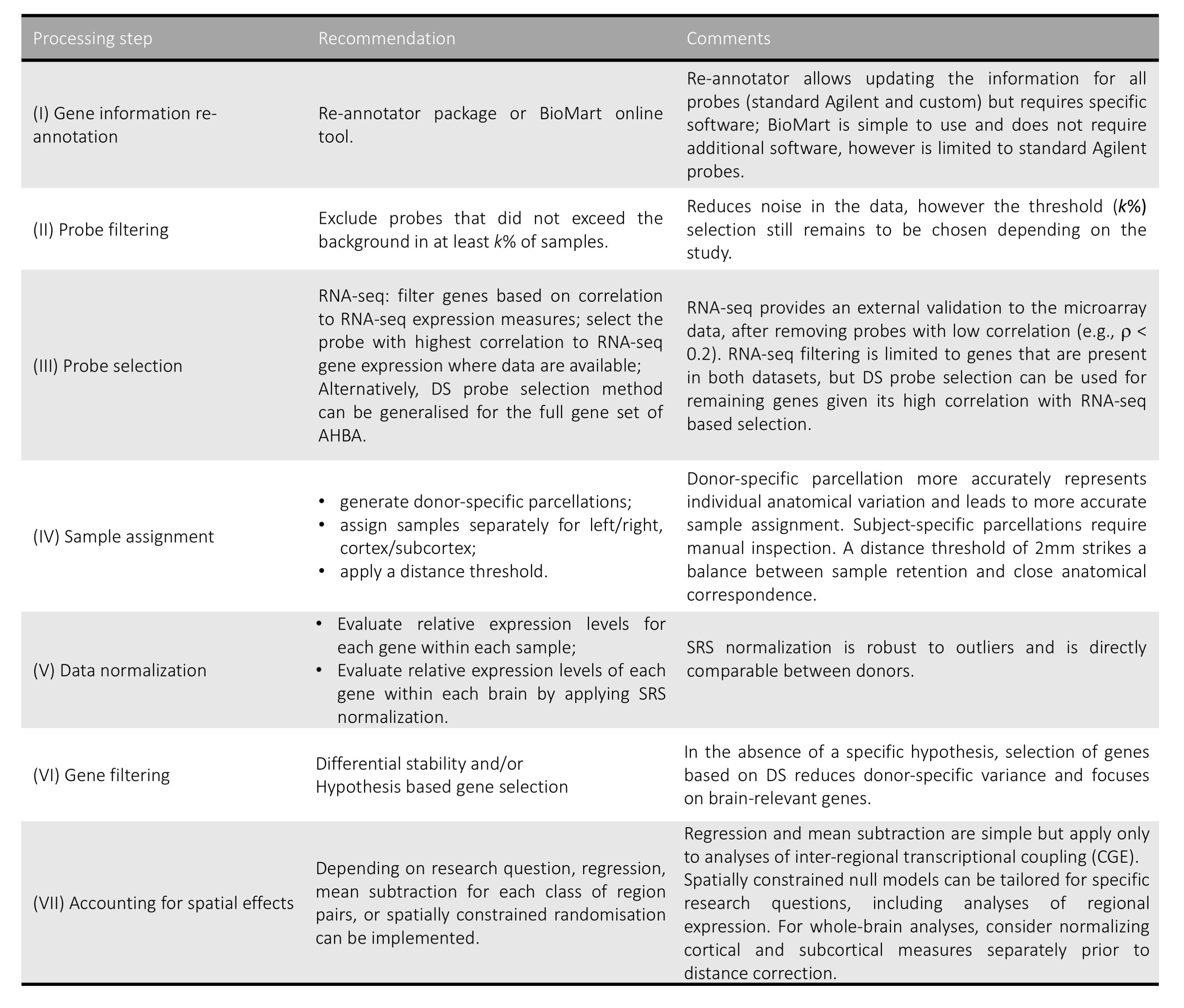
该处理流程根据该文献所述,结合王亚平报告所写
原理
总体流程
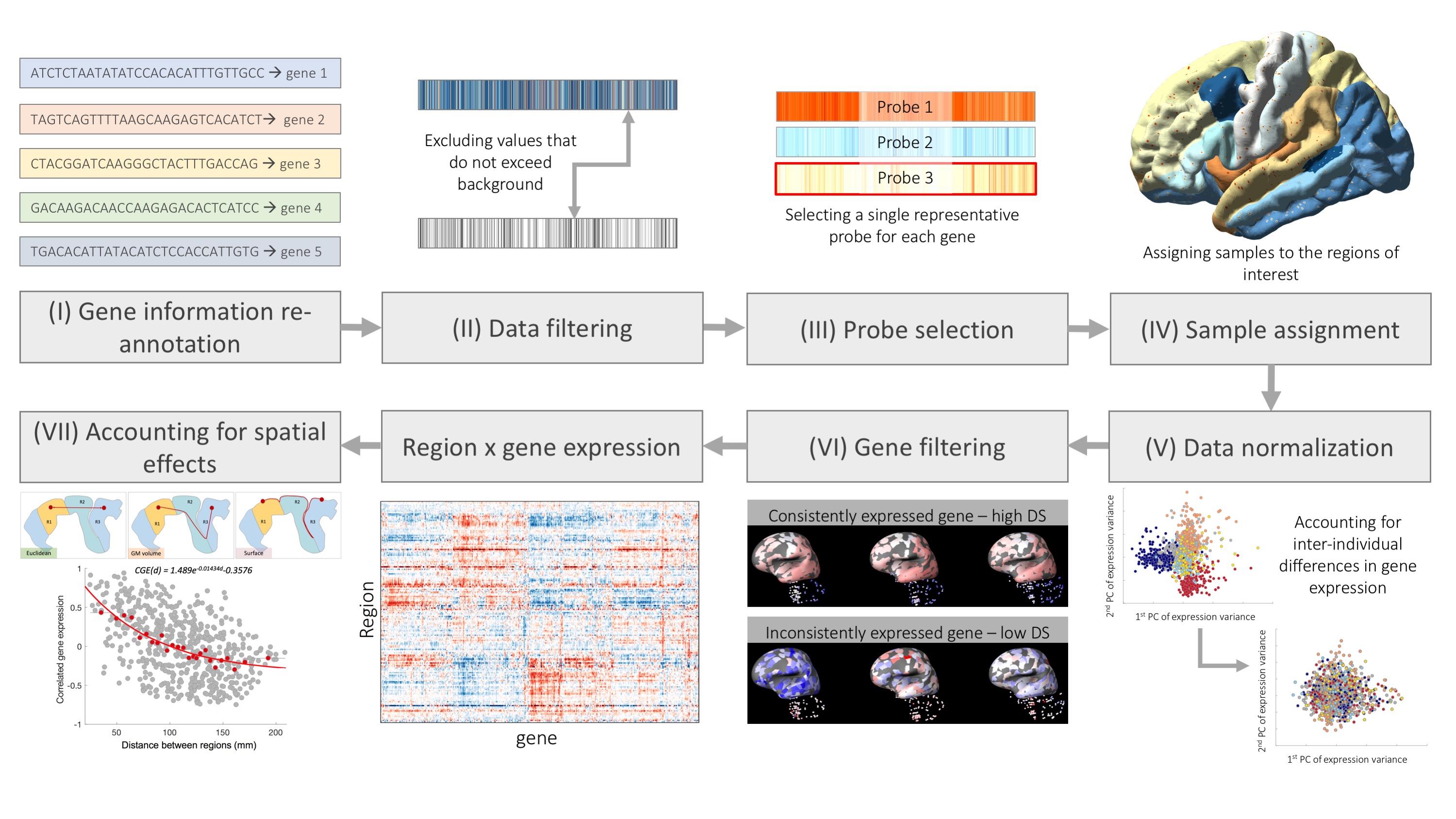
1. 探针重注释
一个基因可以有多个探针来检测,而一个探针通常只对应一个基因,在AHBA中,93%的已知基因至少有两个探针,所以首先要把探针和基因的关系对应上。同时,随着探针和基因对应关系的更新,仅在2013年就有18%的探针不再对应任何基因,故第一步是确定和更新探针到基因的注释。
此步引入外部标准文件:Homo_sapiens.gene_info.gz
附:18年所做的一项重注释的结果,可以看到差异很大
We found that 45,821 probes (78%) were uniquely annotated to a gene and could be related to an entrez ID.
A total of 19% of probes were not mapped to a gene, and just under 3% were mapped to multiple genes and could not be unambiguously annotated.
Of the probes that were unambiguously annotated to a gene, 3438 (7.5%) of the annotations differed from those provided by the AHBA: 1287 probes were re-annotated to new genes and 2151 probes that were not previously assigned to any gene in the AHBA could now be annotated.
Additionally, 6211 (∼ 10%) probes in the initial AHBA dataset had an inconsistent gene symbol, ID or gene name information according to the NCBI database, as of 5th March 2018
2. 数据清洗
基因芯片容易出现一些非特异性的结合,而这将导致最后的结果不准确,鉴于基因芯片的局限性,解决办法是将低于背景噪声的部分直接去除掉。
此步涉及到一个跟基因芯片相关的二进制质控文件
据文章中表述,如不进行清洗,会有约超过22%的基因在至少一半的样本中携带者背景噪声
if we exclude probes that did not exceed the background in at least 50% of all cortical and subcortical samples across all subjects, we exclude 30% of probes (13,844 out of 45,821), assaying 4486 out of 20,232 genesIn other words, if no filtering is performed, > 22% of genes will have expression levels consistent with background noise in at least half of the tissue samples
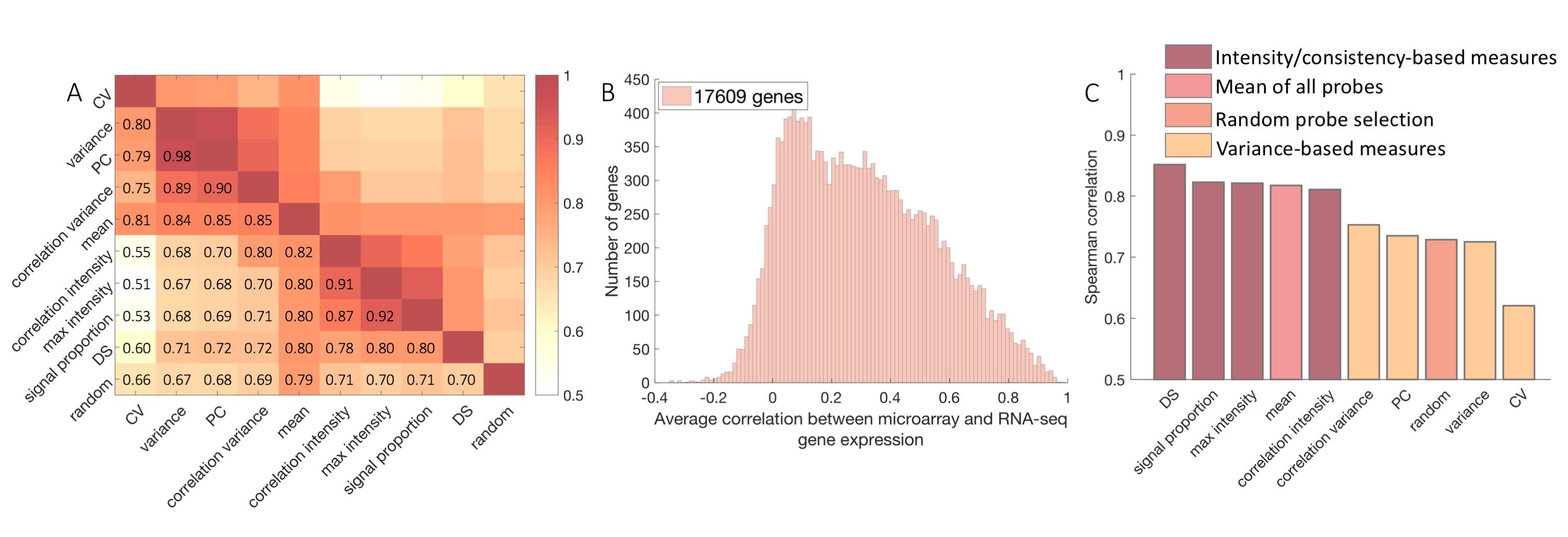
3. 探针选择
由于同一基因对应多个探针,需要对其中一个探针或对多个探针进行平均等不同的方法来定义基因的表达量
在清洗结束后会有71%的基因有至少两个探针(对比原本93%),而即使清洗过后,同一基因的不同探针相关性仍很低
根据作者所述,DS法可能更佳,而根据如图的结果,max和mean也是不错的方法
4. 样本映射到脑区
AHBA提供了每个样本的基于MNI的坐标以及MRI数据,但AHBA的2个大脑是颅内扫描,另外4个是颅外扫描,所以配准过程不一致。文章采用对每个大脑单独应用一种分割方案,对皮层区域进行surface的分割和归一化,对非皮层进行volume的分割和归一化。
对于assign的过程,要注意避免左脑的样本映射到右脑,或者皮层下的样本映射到皮层上,同时推荐使用2mm的阈值进行限制
5. 数据归一化
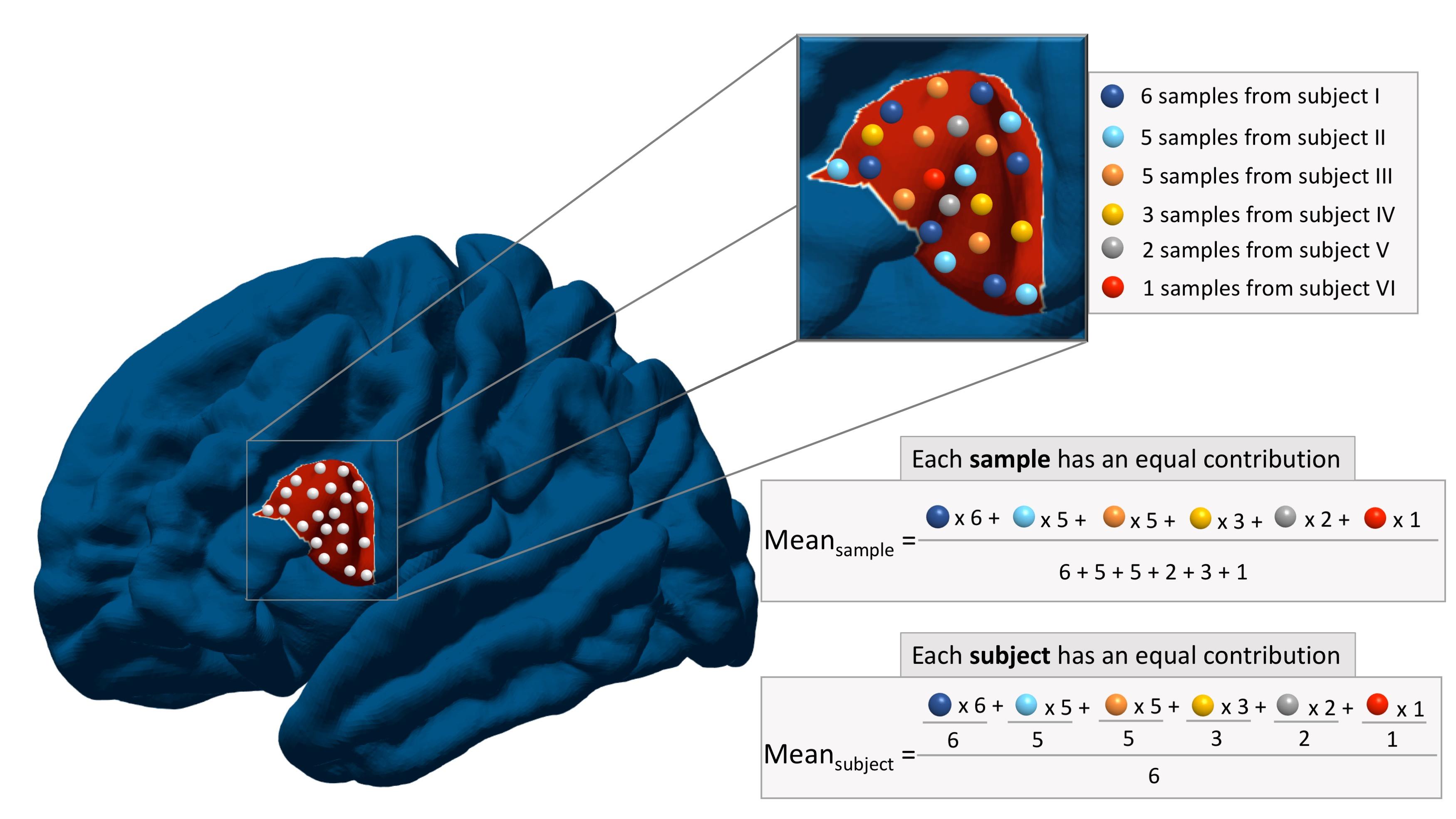
根据"arnatkeviciute_practical_2019"文章的描述,即使AHBA做了归一化,在同一脑的样本间基因表达很相似而不同脑的样本间仍存在较大差异,故认为应当进行再次的归一化,消除个体间的差异。文章中讨论了多种方法,感兴趣可以阅读原文。
根据文章所述,推荐两种方法,视研究者的偏好所定:
- 将一个区域内的所有样本进行平均
- 在个体水平进行平均再汇总
6. 基因筛选
将在不同大脑中表达不一致的基因进行评估、剔除,或提取研究所需的部分基因用于进一步分析
7. 去除空间效应
基因在空间上的相似和不同本身就代表了一定的生物学意义,但在"arnatkeviciute_practical_2019"这篇文章中的观点是
“Although this spatial autocorrelation is, in itself, an important neurobiological feature of the brain transcriptome (Gryglewski et al., 2018), it is critical for any analysis claiming a specific association between spatial variations in gene expression and a given IDP to show that the association exceeds what would be predicted by lower-order spatial gradients of gene expression.” (Arnatkeviciute 等。, 2019, p. 5)
8. 总结
实际操作
"arnatkeviciute_practical_2019"提供了一套相应的代码, 基于Matlab
"markello_standardizing_2021"根据上述论文的步骤提供了开源工具包abagen (documentation)
abagen
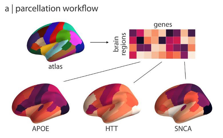
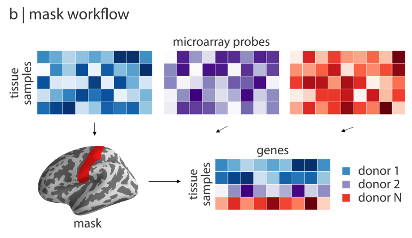
abagen支持两种工作流:
- 输入atlas(默认DesikanKilliany),输出分割后的预处理的区域基因表达矩阵
- 输入mask,输出包含mask的所有预处理过的所有样本的表达数据
同时其运行模式也分为两种,一种是命令行,一种是以python包的形式:
-
Command Line
-
下载数据
该处文档所描述的方法和实际代码是一致的,但实际运行会有各种错误,建议python形式下载或直接拷贝一份
abagen -v --donors all --data_dir $HOME/abagen-data --n_proc 6 atlas #--donors (i.e., 9861, 10021) or UIDs (i.e., H0351.2001) #--n_proc 下载线程数 -
处理数据
为尽量保障最终处理数据的一致性,建议均使用默认参数
abagen -v \
     --ibf_threshold 0.5 \
     --probe_selection diff_stability \
     --lr_mirror None \
     --sim_threshold None \
     --missing None \
     --tol 2 \
     --sample_norm srs \
     --gene_norm srs \
     --norm_all \
     --region_agg donors \
     --agg_metric mean \
     --output-file $PWD/abagen_expression.csv \
     --save-counts \
     --save-donors \
     atlas
#--ibf_threshold  probe超过背景噪音的阈值,单位%
#--probe_selection    选择作为代表基因的探针
#--lr_mirror      由于6个患者中有4个只有左脑数据,是否进行镜像
#--sim_threshold  关联度过滤阈值
#--missing            如何处理没关联上样本的区域
#--tol                匹配到分区的距离阈值
#--sample_norm        样本间归一化表达矩阵的方法
#--gene_norm      基因间归一化表达矩阵的方法
#--norm_all           归一化的范围是否为全部样本而不是match到脑区的样本
#--norm_structures    归一化的范围是否为结构之间而不是全部样本
#--region_agg     当多个样本匹配到同一区域时先患者内部合并还是一起合并
#--agg_metric     合并方法
#--no-reannotated 是否不要重注释探针, 为进行重注释
#--no-corrected-mni   用原始MNI坐标系还是用alleninf修正后的坐标系,False为用修正后的
-
-
Python
-
下载及加载数据
import abagen
#下载所有数据至$HOME/abagen-data/microarray,约4G
#可从    上导入
#files = abagen.fetch_microarray(donors='all')
#加载已下载好的数据,abagen.io提供了对数据文件的操作(详见文档)
files = abagen.fetch_microarray(donors=['12876', '15496'], data_dir='/path/to/my/data/')
数据结构
/path/to/my/data/ ├── normalized_microarray_donor10021/ │ ├── MicroarrayExpression.csv │ ├── Ontology.csv │ ├── PACall.csv │ ├── Probes.csv │ └── SampleAnnot.csv ├── normalized_microarray_donor12876/ ├── normalized_microarray_donor14380/ ├── normalized_microarray_donor15496/ ├── normalized_microarray_donor15697/ └── normalized_microarray_donor9861/ -
分割脑区
#可接受MNI、fsaverage/fsaverage5、 Desikan-Killiany等模板空间
atlas = abagen.fetch_desikan_killiany()
#返回的atlas有两个属性,一个是image包含atlas数据的图像文件路径,一个是info包含关于分割的额外信息的csv文件路径
-
matlab(弃坑)
https://github.com/BMHLab/AHBAprocessing
环境配置
前置工具箱
- Brain Connectivity Toolbox, Version 2017-15-01.
- Toolbox Fast Marching, Version 1.2.0.0
数据说明
数据文件存放在this figshare repository,根据文件说明,仅包含左脑皮层处理后的数据,其他数据需要自行计算。
AHBAprocessed
在这部分数据分别分别包含:
-
在左脑的处理中经过如下筛选仅剩下10 027个基因:
- 探针注释采用的Re-Annotator包
- 移除在超过一半的样本中都没有高于背景噪音的探针
- 移除RNA-seq中未出现的基因
- 移除与RNA-seq中低相关性的探针
- 根据RNA-seq的结果选择最高相关性的探针
结果
- ROIxGene_aparcaseg_RNAseq.mat
34 ROIs per hemisphere: mean 37.8 ± 22.5 (SD) samples assigned per ROI, min= 5; max = 92;
No regions have been excluded. - ROIxGene_cust100_RNAseq.mat
100 ROIs per hemisphere: mean 7.4 ± 6.5 (SD) samples assigned per ROI, min= 0; max = 37;
Region 54 has been excluded. - ROIxGene_cust250_RNAseq.mat.
250 ROIs per hemisphere: mean 5.1 ± 3.5 (SD) samples assigned per ROI, min= 0; max = 18;
Regions 122, 127, 180, 183, 223, 230 have been excluded. - ROIxGene_HCP_RNAseq.mat
180 ROIs per hemisphere: mean 7.1 ± 6.7 (SD) samples assigned per ROI, min= 0; max = 41;
Regions 23, 89 and 104 have been excluded.
-
在以下的筛选中得到15 745个基因:
- 探针注释采用的Re-Annotator包
- 移除在超过一半的样本中都没有高于背景噪音的探针
结果
- ROIxGene_aparcaseg_INT.mat
34 ROIs per hemisphere: mean 37.8 ± 22.5 (SD) samples assigned per ROI, min= 5; max = 92;
No regions have been excluded. - ROIxGene_cust100_INT.mat
100 ROIs per hemisphere: mean 7.4 ± 6.5 (SD) samples assigned per ROI, min= 0; max = 37;
Region 54 has been excluded. - ROIxGene_cust250_INT.mat
250 ROIs per hemisphere: mean 5.1 ± 3.5 (SD) samples assigned per ROI, min= 0; max = 18;
Regions 122, 127, 180, 183, 223, 230 have been excluded. - ROIxGene_HCP_INT.mat
180 ROIs per hemisphere: mean 7.1 ± 6.7 (SD) samples assigned per ROI, min= 0; max = 41;
Regions 23, 89 and 104 have been excluded.
AHBAdata
分别包含:
-
分割
- 对6个患者均包括了四种分割方式
- defaultparc_NativeAnat.nii
34 regions per hemisphere + 7 subcortical regions; Desikan et al, 2006. - random200_acpc_uncorr_asegparc_NativeAnat.nii
100 random regions per hemisphere + 10 subcortical regions. - HCPMMP1_acpc_uncorr.nii
180 regions per hemisphere; Glasser et al., 2016. - random500_acpc_uncorr_asegparc_NativeAnat.nii
250 random regions per hemisphere + 15 subcortical regions.
- defaultparc_NativeAnat.nii
- 每种分割方式均包含了左脑皮层的Annotation文件
- lh.aparc.annot
- lh.random200.annot
- lh.HCP-MMP1.annot
- lh.random500.annot
- FreeSurfer的average模板中左脑皮层白质和灰质的surfaces
- lhfsaverage.pial
- lhfsaverage.white
- 左脑皮质surface的球形展示
- lh.sphere
- HCPMMP1在MNI木板上的volume分割
- MMPinMNI.nii
- 对6个患者均包括了四种分割方式
-
探针重注释
- hba_microarray_probes_fixed.xlsx
一部分基因名被excel格式化需要手动更改 - probes2annotateALL.fasta
Re-annotator所需要的注释文件 - probes2annotateALL_merged_readAnnotation.txt
Re-annotator注释的输出文件
- hba_microarray_probes_fixed.xlsx
-
处理后的数据
- 为defaultparc_NativeAnat分割预先计算的在皮层surface和灰质volume的样本间距离
- 预先计算的在不同探针选择方法过滤前和过滤后的相关性
-
原始数据
从AHBA下载的未处理的基因表达数据和一些预处理的数据如:
-
reannotatedProbes.mat
用Re-annotator软件包重注释的探针矩阵
-
Probes.xlsx
由AHBA提供的探针信息包括名字、ID、相关基因信息
-
mart_export_updatedProbes.txt
用biomart注释的探针,limmanormalisedExpression.txt使用limma归一化的基因表达数据
-
代码解读
-
AddPaths.m
添加当前文件夹的所有子目录到matlab
-
processingPipeline.m
这个文件下的配置是最主要的部分,详见README_processingPipeline.txt
此步需要自行下载最新的注释文件
clear all; close all; options = struct(); #是否排除小脑和脑干 options.ExcludeCBandBS = true; #是否使用CUST探针 options.useCUSTprobes = true; #reannotator或Biomart #该步的更新需要手动更新相应的文件 #mart_export_updatedProbes.txt in data/genes/rawData #reannotatedProbes.mat in data/genes/rawData options.updateProbes = 'reannotator'; #探针选择标准 #Variance, RNAseq, PC, maxIntensity, maxCorrelation_intensity, maxCorrelation_variance, CV, LessNoise, Mean, Random, DS options.probeSelections = {'RNAseq'}; #分割模板 #'HCP': 180 nodes per hemisphere #'aparcaseg': 34 nodes per hemisphere + subcortex #'cust100': 100 nodes per hemisphere + subcortex #'cust250': 250 nodes per hemisphere + subcortex options.parcellations = {'aparcaseg'}; #'ontology' - samples are separated into cortical and subcortical based on AHBA ontology information #'listCortex' - samples are separated into cortical and subcortical based on re-defined list of region names; options.divideSamples = 'listCortex'; #映射是否排除海马 options.excludeHippocampus = false; #映射分配阈值 options.distanceThreshold = 2; #超过背景噪音的阈值,单位% options.signalThreshold = 0.5; #基于方差的过滤 options.VARfilter = false; options.VARscale = 'normal'; options.VARperc = 50; options.RNAsignThreshold = false; options.RNAseqThreshold = 0.2; options.correctDistance = false; options.calculateDS = true; options.distanceCorrection = 'Euclidean'; options.Fit = {'exp'}; options.normaliseWhat = 'Lcortex'; options.normMethod = 'scaledRobustSigmoid'; options.percentDS = 100; options.doNormalise = true; options.saveOutput = true; options.normaliseWithinSample = true; options.xrange = [0 220]; options.plotCGE = true; options.plotResiduals = true; options.meanSamples = 'meanSamples'; -
S[1-4]_*.m
- S1_extractData.m
- S2_probes.m,选择探针
- S3_samples2parcellation.m,样本映射到脑区
- S4_normalisation.m,归一化数据,制作region x gene和CGE矩阵
研究角度
Allen的基因数据处理后得到的结果形式是region x gene的一个矩阵,内部的值为基因的表达量,是一个相对值,即不能进行绝对值相关的研究
根据我们的研究方向,很自然就首先联想到基因的偏侧化差异,但不幸的是,根据Allen团队的叙述,基因在半球间没有统计学显著的差异,这与一些神经发育的研究结果吻合。
“Interestingly, no statistically significant hemispheric differences could be identified at this fine structural level that were corroborated in both brains (paired one-sided t-tests, P , 0.01, BenjaminiHochberg (BH)-corrected)” (Hawrylycz 等。, 2012, p. 393) (pdf)
“Preliminary analyses of these data revealed minimal lateralization of microarray expression, and so samples were collected exclusively from the left hemisphere for the following four donors” (Markello 等。, 2021, p. 15) (pdf)
下图能够很好地说明我们可能用到的研究角度,以下说明围绕此图进行阐述
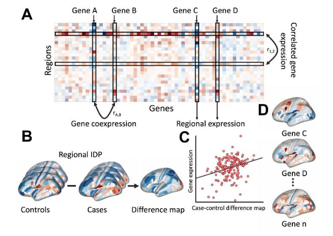
基因差异分析
最基础的角度,我们可以通过比较不同的分组之间的基因表达情况来得出最直接的结果,而分组的角度可以是多维的,从临床、行为、脑影像等方面,比较的基因也可以是一组基因、全部基因。如:
- 额叶和顶叶之间的基因表达差异、灰质和白质的基因表达差异、FA高表达和FA低表达区域的基因表达差异
- 男性和女性海马区的基因表达差异
- gene A高表达和gene A低表达区域的(其他)基因表达差异
- 在组间进行GSEA分析,即不同分组间的基因富集差异
- WGCNA
- ……
而在得到差异基因之后,就可以进行进一步的分析
- 我们可以做出一些图来表示出这些差异基因的占比、差异程度、正向反向等信息
- 对这些差异基因进行富集分析,看看这些基因都在哪些通路上,即这些差异基因都执行了什么功能
- 以差异程度做GSEA分析,即差异的基因在哪些通路上的贡献比较大
- GSVA
- PPI分析
基因共表达
由于基因执行功能的不同,故基因在空间上的分布也不尽相同,从而出现分布上的特征,而与其功能密切相关的基因通常也会呈现出与该基因的相关性(正向或反向)。
基因共表达研究的是gene A与gene B是否在空间的分布上存在相关性
相关基因表达
当我们研究某项影像学指标时,如果在不同位置上出现一致性,一定会好奇其内在的基因表达上是否也一致,而相关基因表达便是测量不同位置上的基因表达谱是否存在相关性
而当上述思路进行推广可得全脑区的基因表达谱相关性热图,即region x region的矩阵,值为相互间的基因表达谱相关性,若在此基础上结合其他脑影像指标的区域间相关性热图的region x region矩阵,便可相结合进行该指标与基因表达谱之间的相关性,即该指标的变化是否与一组基因相关。